Getting started with mpeccable

This section will describe some of the basic components of mpeccable. We are going to define a functional, a control variable. We then put them in a constraint and show how we can extract the levels and jacobian for a given value of the parameters.

The problem

We consider an extremely simple problem of asset accumulation with some level of uncertainty. We consider 3 state of the world index by z. In state z the agent recieved z amounts of apple.

Each period the agent decides how much to consume and how much to save. The agent discounts the future at rate $ r$ and earns the same interest on savings. We use CRRA utility function.

The dynamic problem is simply represented using $ V_z(): $ implicitely defined by the following Bellman equation:

\[ V_z(a) = \max_{a'} u((1+r) a + z -a') + \frac{1}{1+r} E_{z'|z} V_{z'}(a') \]

The collocation

First we define the collocation. This is a list of values at which the constraint should be evaluated. At this point we do something very simple, we define uniform grid between on $ [0,1] $ and discretize it over 10 points. We also choose 3 discrete states for the variable \(z\).

require(mpeccable)

Na = 10
asupp = seq(0, 1, l = Na)
zvals = 1:3
cc = expand.grid(a = asupp, z = zvals)

Create a functional

Creating the functional representation of the value function is very simple thanks to the utility functions that create specific ones for you. For example, F_SplineInt1D generates a 1-dimensional spline indexed by an integer. This is perfect to represent our value $ V_z(a)$.

V = F_SplineInt1D(asupp, zvals)
g. = param0(V, "g", 1)

The second line collects an itinialized parameter vector that represents a particular $ V_z(a)$ function. g. is of type FDiff, its levels are the coefficients of the representing spline. Here we have 12 of them. The Jacobian is 12x12 and diagonal. V is of type frep and that's why we were able to call params0 on it which returns the an itinialized parameter vector.

Create a control variable

Remember that in our problem we have to optimaly choose the asset in the next period. This is a control variable and we need to declare it since we want to compute the Jacobian with repsect to it.

a_ = FDiff(cc$a - 0.1, "a")

Using the FDiff function I can easily do that and generate this control variable. I gave it the label a and use an underscore as a naming convention for my code. I tell the function that this control variable must be chosen at each asset a in the collocation. In another document we'll show that generalizes to multiple dimensions.

Our first Jacobian

We can now look at the Jacobian of the value function evaluated at the control variable:

options(mpeccable.coloring = TRUE)
R = V(a_, cc$z, g.)
image(R@J)

plot of chunk simpleplot

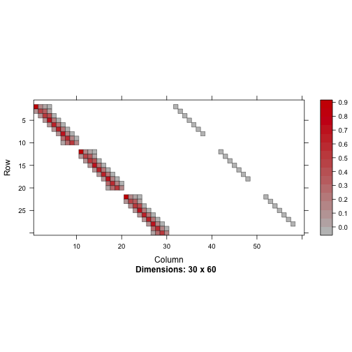
First we called options(mpeccable.coloring=TRUE) to tell mpeccable that we don't want th actual values of the Jacobian, but we just want to know what parts are potentially non zero. The right of the figure contains a diagonal matrix. This represents the derivative of $ V $ with respect to the control variables \(a^*_j\). There is exactly one control per state \((a_j,z_j)\). Then the left part has big blocks. This is because the control the spline is evaluated at the control variable for which we don't know ex-ante the value. Because the optimizer needs to know the structure from the begining, we need to be conservative and allow for any parameter of the spline to be entering a given state. However, some sparisty remains, because we know for sure that a $ a_j$ from a given $ z_j$ never enters a different $ z_j$ hence the lbock diagonal.

Define the utility and the low of motion for z

We choose a simple utilty CRRA utility function with parameter $ 0.5$ and we use interest rate of 5%

U = ((1 + 0.05) * cc$a - a_)^0.5
Up = 0.5 * ((1 + 0.05) * cc$a - a_)^(1 - 0.5)

For simplicity, assumes that z goes in circle, from 1, to 2, to 3 and back to 1, I can define z tommorow as:

z1 = (cc$z%%3) + 1

And using this z1 I can write up the Bellman level constraint:

R = V(cc$a, cc$z, g.) - U - 0.95 * V(a_, z1, g.)
image(R@J)

plot of chunk simpleplot2

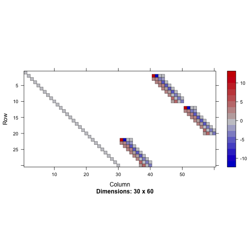
And this is the Jacobian for our Bellman equation, now we need to add the first order condition and we are done! Notice how now the function parameters also appear in the contemporaneously through the diagonal because of the first term.

First order condition, Euler equation

The last equation we need to garantee optimally, is the first order condition.

\[ u'((1+r) a -a') = \frac{1}{1+r} E_{z'|z} V'_{z'}(a') \]

R2 = Up - 0.95 * V(a_, z1, g., deriv = 1)
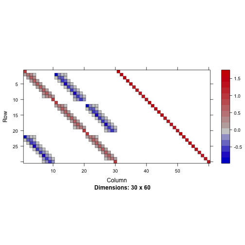
image(R2@J)

plot of chunk simpleplot3

Combine all the constraints

R2 = Up - 0.95 * V(a_, z1, g., deriv = 1)
image(R@J)

plot of chunk simpleplot4